Bookmarked Websites

Udemy has many courses related to data science, machine learning and programming. Many of the courses are also approved by SkillsFuture Singapore.
Loop (Frontiers) is a research network that is open to be integrated into any publisher’s or academic organization’s website. It can also collate a list of publications by a researcher automatically, similar to Google Scholar or ResearchGate.
Frontiers Loop Profile Page
Kaggle is very useful for finding datasets. Kaggle also provides (limited) free access to GPUs, which is helpful for deep learning.
Kaggle Profile Page
ResearchGate is a European commercial social networking site for scientists and researchers to share papers, ask and answer questions, and find collaborators. One advantage is that sometimes authors upload their preprint PDFs onto ResearchGate, which can be viewed for free.
ResearchGate Profile Page
ScholarBank@NUS is the institutional repository of the National University of Singapore. It stores the scholarly output of NUS, including students’ academic theses.
ScholarBank Profile Page
GitHub is a popular code hosting platform for version control and collaboration.
GitHub Profile Page
NUSMods is a very useful website for NUS students to plan their academic timetable, for lectures, tutorials and exams.
An example is this MA1513 Linear Algebra Timetable for a module that I previously helped to teach.
Math Genealogy is a website that traces a mathematician’s academic genealogy, meaning the PhD supervisor of one’s PhD supervisor, and so on, all the way back to the earliest history.
Math Genealogy Profile Page
Publons is a unique website that provides a free service for academics to track, verify, and showcase their peer review and editorial contributions for academic journals. It is owned by Clarivate Analytics (which also owns Web of Science, EndNote, and ScholarOne).
Publons Profile Page
Microsoft Academic is a free public web search engine for academic publications and literature, developed by Microsoft Research. In terms of functionality, it is similar to Google Scholar.
Microsoft Academic Profile Page
Scopus is Elsevier’s abstract and citation database covering various publishers and peer-reviewed journals.
Scopus Profile Page
Google Sites is a free web page-creation tool offered by Google.
Google Sites Page

When to use Variation of Parameters / Method of Undetermined Coefficients

There are two methods to solve 2nd order linear Non-homogenous D.E.: Variation of Parameters and Method of Undetermined Coefficients. (see this notes for details)

A common question is: when to use which method?

Simple Guideline: If $r(x)$ (the right-hand side of the D.E. $y''+p(x)y'+q(x)y=r(x)$ ) is a

Polynomial
Exponential ( $e^{kx}$ )
Sine or Cosine ( $\sin kx$ or $\cos kx$ )
Or combinations of the above

use Method of Undetermined Coefficients for fast solution. Note: It is 100% correct to use Variation of Parameters for the above cases, but it is usually slower due to the integration involved.

For all other cases not covered above, use Variation of Parameters.

Examples from Midterm

(2016 Q10) $y''-2y'-3y=4e^x+4e^{3x}$ . Use Method of Undetermined Coefficients since $r(x)$ is a sum of exponential functions.

(2015 Q9) $y''+4y=\cos 2x$ . Use Method of Undetermined Coefficients since $r(x)$ is a cosine function.

(2015 Q10) $y''-4y=e^{x^2}$ . Although $r(x)=e^{x^2}$ is an exponential, it is not of the form $e^{kx}$ . Also, the fact that $A(x)$ and $B(x)$ are integrals clearly suggests that they are related to the $u,v$ in the method of Variation of Parameters. So we use Variation of Parameters.

(2014 Q10) $y''-2y'+y=e^x\cosh x$ . On the surface, $e^x\cosh x$ does not fall into the category of polynomial/exponential/cos/sine, so we use Variation of Parameters as shown in the official answer.

However, if we know the identity $\cosh(x)=\frac 12(e^x+e^{-x})$ , we can actually rewrite the equation as $y''-2y'+y=\frac 12 e^{2x}+\frac 12$ and use Method of Undetermined Coefficients.

Outline of solution using Method of Undetermined Coefficients:

Guess $y_p=Ae^{2x}+B$ . Then $y_p''-2y_p'+y_p=Ae^{2x}+B$ , where we can clearly see that $A=B=\frac 12$ . Then $y=c_1e^x+c_2xe^x+\frac 12 e^{2x}+\frac 12$ . Upon plugging in the initial conditions, we find that $c_1=c_2=1$ .

Hence $y(2)=e^2+2e^2+\frac 12 e^4+\frac 12=49.966\approx 50$ .

The Brachistochrone

Entertaining video to (hopefully) increase your interest in math.

Recently, I saw this video in the “Trending” section of YouTube (3 million views). It is actually related to differential equations.

The basic question behind this is: What is the shape of the curve that will allow a ball to slide frictionlessly (under gravity) to a given end point in the shortest time? Rather surprisingly, the answer is not a straight line, even though a straight line is the shortest distance between two points.

Perhaps even more surprising is that such a curve is a tautochrone curve, where the time taken by an object sliding without friction in uniform gravity to its lowest point is independent of its starting point

Note: Do not worry, this is not tested.

Limit Question

Question: What is the value of

$\displaystyle\lim_{x\to 0}\frac{e^{-1/x^2}}{x}$

Solution: limit-solution

This question is not very difficult, but involves a trick. Feel free to try it and discuss with your friends.

If you managed to solve it, you can email me and I will post the first correct answer (with working) here.

Otherwise I will post the solution at the end of next week.

Hope you have fun solving this. 🙂

Line integral over a scalar field f

line_integral_of_scalar_field

The line integral over a scalar field f can be thought of as the area under the curve C along a surface z = f(x,y), described by the field.

The above graph is a contour plot, where different colors are used to denote different values of f(x,y); in this case the redder colors are used to indicate higher values, bluer colors are used to indicate lower values.

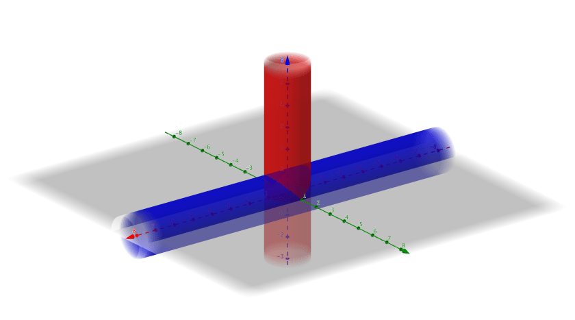
Source: https://en.wikipedia.org/wiki/Line_integral

3d Plots (Tutorial 8)

Q2) Steinmetz solid

q2 cylinder.png

Q3)

sphere-q3

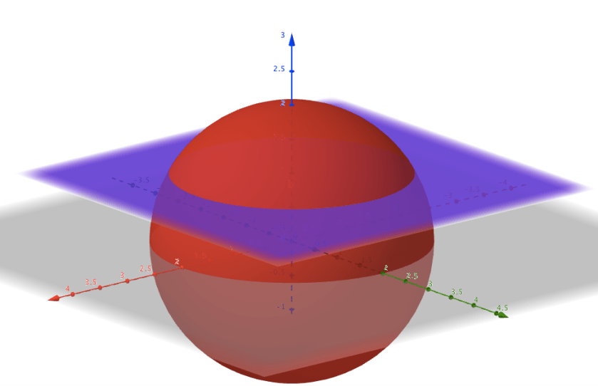
Q4)

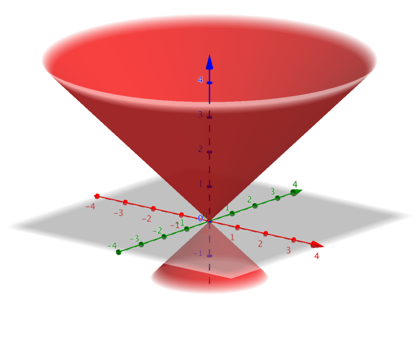
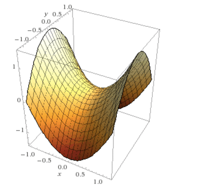
This is the double cone $z^2=x^2+y^2$ . The upper cone is the part above the xy-plane.

double cone Q4.png

Q6) Saddle surface $z=x^2-y^2$

saddle-surface

Visualizing Double Integrals

For beginners, Double Integrals can be difficult to visualize as the resulting diagram is in 3 dimensions. Here are some resources that can help:

1) YouTube Animation

This excellent animation explains the concept behind double integration and also polar integrals.

2) Wolfram Alpha Command: 3dplot

This command can help to visualize the surface $z=f(x,y)$ . For example, in Tutorial 7 Q3, what does the surface $z=x$ looks like?

You can type “3dplot z=x” into WolframAlpha: http://www.wolframalpha.com/input/?i=3dplot+z%3Dx

Result:

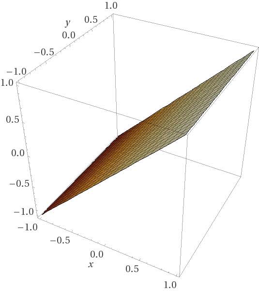
This makes sense, since $z=x$ means $x-0y-z=0$ , i.e. we can see that the surface should be a plane.

Lagrange Multiplier Summary

The method of Lagrange Multipliers can be summarized in one single formula:

$\huge\boxed{\nabla f=\lambda\nabla g}$

where $f$ is the function to be optimized and $g=0$ is the constraint.

Example

Let’s illustrate this using the example in your notes (pg 40): Find the relative extrema of $f(x,y)=12x-16y+50$ subject to the constraint $x^2+y^2=25$ .

Let $g(x,y)=x^2+y^2-25$ denote the constraint. According to the formula $\boxed{\nabla f=\lambda\nabla g}$ ,

$\begin{pmatrix}f_x\\f_y\end{pmatrix}=\lambda\begin{pmatrix}g_x\\g_y\end{pmatrix}$

$\begin{pmatrix}12\\-16\end{pmatrix}=\lambda\begin{pmatrix}2x\\2y\end{pmatrix}$

Now we need to solve the simultaneous equations: $12=\lambda 2x$ , and $-16=\lambda 2y$ , and the constraint $x^2+y^2=25$ .

From this part onwards, the solving is identical to the part in the notes.

To understand Lagrange Multiplier intuitively, check out this nice post on Quora.

Ratio Test and Radius of Convergence

The following is an excellent video on how to find radius of convergence using Ratio Test by Khan Academy. Tip: If the speech is too slow, you may want to adjust to 2x speed on YouTube.

The rigorous proof of the Ratio Test requires the formal definition of limit, taught in e.g. MA2108 Mathematical Analysis I.

The rough idea is that $\displaystyle\lim_{n\to\infty}|\frac{a_{n+1}}{a_n}|<1$ means that for large $n$ onwards, the series is (less than) a geometric progression with common ratio $|r|<1$ , which is known to converge. Thus the series itself converges.

To learn more about the proof, you may want to check out this webpage.

Fundamental Theorem of Calculus (Part I)

For Tutorial 2 Q3, we are actually using Part 1 of the Fundamental Theorem of Calculus, which states that $\displaystyle\frac{d}{dx}\int_a^x f(t)\,dt=f(x)$ for a continuous function $f$ .

If the upper limit is a function $g(x)$ instead, we have $\Large\displaystyle\boxed{\frac{d}{dx}\int_a^{g(x)}f(t)\,dt=f(g(x))g'(x)}$ by the chain rule. This is the formula that is going to be useful for Q3.