Limit Question

Question: What is the value of

$\displaystyle\lim_{x\to 0}\frac{e^{-1/x^2}}{x}$

Solution: limit-solution

This question is not very difficult, but involves a trick. Feel free to try it and discuss with your friends.

If you managed to solve it, you can email me and I will post the first correct answer (with working) here.

Otherwise I will post the solution at the end of next week.

Hope you have fun solving this. 🙂

Line integral over a scalar field f

line_integral_of_scalar_field

The line integral over a scalar field f can be thought of as the area under the curve C along a surface z = f(x,y), described by the field.

The above graph is a contour plot, where different colors are used to denote different values of f(x,y); in this case the redder colors are used to indicate higher values, bluer colors are used to indicate lower values.

Source: https://en.wikipedia.org/wiki/Line_integral

3d Plots (Tutorial 8)

Q2) Steinmetz solid

q2 cylinder.png

Q3)

sphere-q3

Q4)

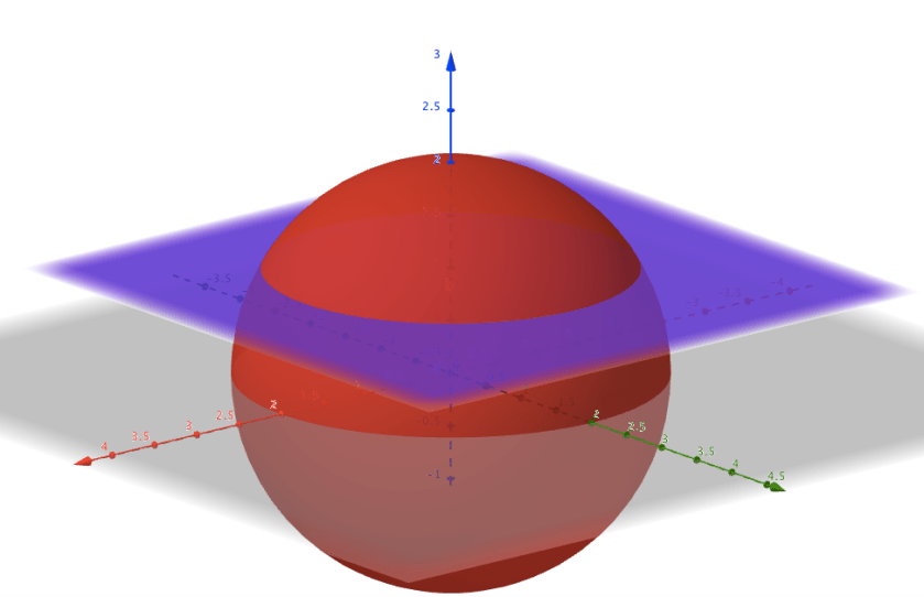
This is the double cone $z^2=x^2+y^2$ . The upper cone is the part above the xy-plane.

double cone Q4.png

Q6) Saddle surface $z=x^2-y^2$

saddle-surface

Visualizing Double Integrals

For beginners, Double Integrals can be difficult to visualize as the resulting diagram is in 3 dimensions. Here are some resources that can help:

1) YouTube Animation

This excellent animation explains the concept behind double integration and also polar integrals.

2) Wolfram Alpha Command: 3dplot

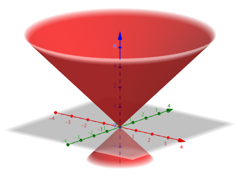
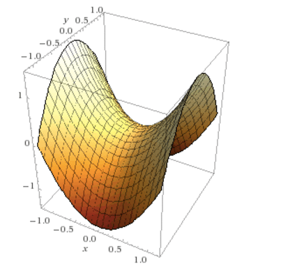
This command can help to visualize the surface $z=f(x,y)$ . For example, in Tutorial 7 Q3, what does the surface $z=x$ looks like?

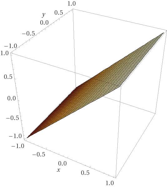
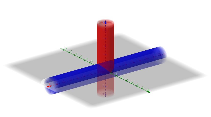
You can type “3dplot z=x” into WolframAlpha: http://www.wolframalpha.com/input/?i=3dplot+z%3Dx

Result:

This makes sense, since $z=x$ means $x-0y-z=0$ , i.e. we can see that the surface should be a plane.

Lagrange Multiplier Summary

The method of Lagrange Multipliers can be summarized in one single formula:

$\huge\boxed{\nabla f=\lambda\nabla g}$

where $f$ is the function to be optimized and $g=0$ is the constraint.

Example

Let’s illustrate this using the example in your notes (pg 40): Find the relative extrema of $f(x,y)=12x-16y+50$ subject to the constraint $x^2+y^2=25$ .

Let $g(x,y)=x^2+y^2-25$ denote the constraint. According to the formula $\boxed{\nabla f=\lambda\nabla g}$ ,

$\begin{pmatrix}f_x\\f_y\end{pmatrix}=\lambda\begin{pmatrix}g_x\\g_y\end{pmatrix}$

$\begin{pmatrix}12\\-16\end{pmatrix}=\lambda\begin{pmatrix}2x\\2y\end{pmatrix}$

Now we need to solve the simultaneous equations: $12=\lambda 2x$ , and $-16=\lambda 2y$ , and the constraint $x^2+y^2=25$ .

From this part onwards, the solving is identical to the part in the notes.

To understand Lagrange Multiplier intuitively, check out this nice post on Quora.

Ratio Test and Radius of Convergence

The following is an excellent video on how to find radius of convergence using Ratio Test by Khan Academy. Tip: If the speech is too slow, you may want to adjust to 2x speed on YouTube.

The rigorous proof of the Ratio Test requires the formal definition of limit, taught in e.g. MA2108 Mathematical Analysis I.

The rough idea is that $\displaystyle\lim_{n\to\infty}|\frac{a_{n+1}}{a_n}|<1$ means that for large $n$ onwards, the series is (less than) a geometric progression with common ratio $|r|<1$ , which is known to converge. Thus the series itself converges.

To learn more about the proof, you may want to check out this webpage.

Fundamental Theorem of Calculus (Part I)

For Tutorial 2 Q3, we are actually using Part 1 of the Fundamental Theorem of Calculus, which states that $\displaystyle\frac{d}{dx}\int_a^x f(t)\,dt=f(x)$ for a continuous function $f$ .

If the upper limit is a function $g(x)$ instead, we have $\Large\displaystyle\boxed{\frac{d}{dx}\int_a^{g(x)}f(t)\,dt=f(g(x))g'(x)}$ by the chain rule. This is the formula that is going to be useful for Q3.

If you are still unsure, you may want to check out this 10 minute video that shows some examples: